Video:
((Lightly edited) slides://www.hdjkn.com/files/factored-set-slide.pdf
((Part 1, Title Slides) · · ·有限的委托集s
(第1部分,动机)···Some Context
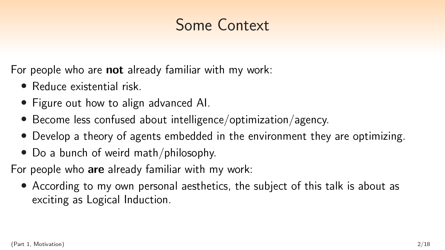 斯科特:So I want to start with some context. For people who are not already familiar with my work:
- 我的主要动机是降低存在风险。
- 我尝试通过弄清楚如何做到这一点艾尔ignadvanced artificial intelligence.
- I try to dothisby trying to becomeless confusedabout intelligence and optimization and agency and various things in that cluster.
- 我这里的主要策略是开发一种代理理论嵌入in the environment that they’re optimizing. I think there are a lot of open hard problems around doing this.
- This leads me to do a bunch of weird math and philosophy. This talk is going to be an example of some weird math and philosophy.
适用于谁是艾尔ready familiar with my work, I just want to say that according to my personal aesthetics, the subject of this talk is about as exciting asLogical Induction,也就是说,我对此感到非常兴奋。我对这次听众感到非常兴奋。我很高兴现在发表这次演讲。
((Part 1, Table of Contents) · · ·考虑说话
 This talk can be split into 2 parts:
第1部分,简短的纯粹组合学谈话。
第2部分,更应用和哲学的主要谈话。
This talk can also be split into5parts differentiated by color:标题幻灯片,,,,Motivation,,,,Table of Contents,,,,Main Body,,,,andExamples。Combining these gives us 10 parts (some of which are not contiguous):
| 第1部分:简短的交谈 | Part 2: The Main Talk | |
| 标题幻灯片 | 有限的委托集s | 这Main Talk (It’s About Time) |
| Motivation | Some Context | 这Pearlian Paradigm |
| Table of Contents | 考虑说话 | We Can Do Better |
| Main Body | Set Partitions,,,,etc. | Time and Orthogonality,,,,etc. |
| Examples | Enumerating Factorizations | Game of Life,,,,etc. |
(第1部分,主体)···Set Partitions
 好的。Here’s some background math:
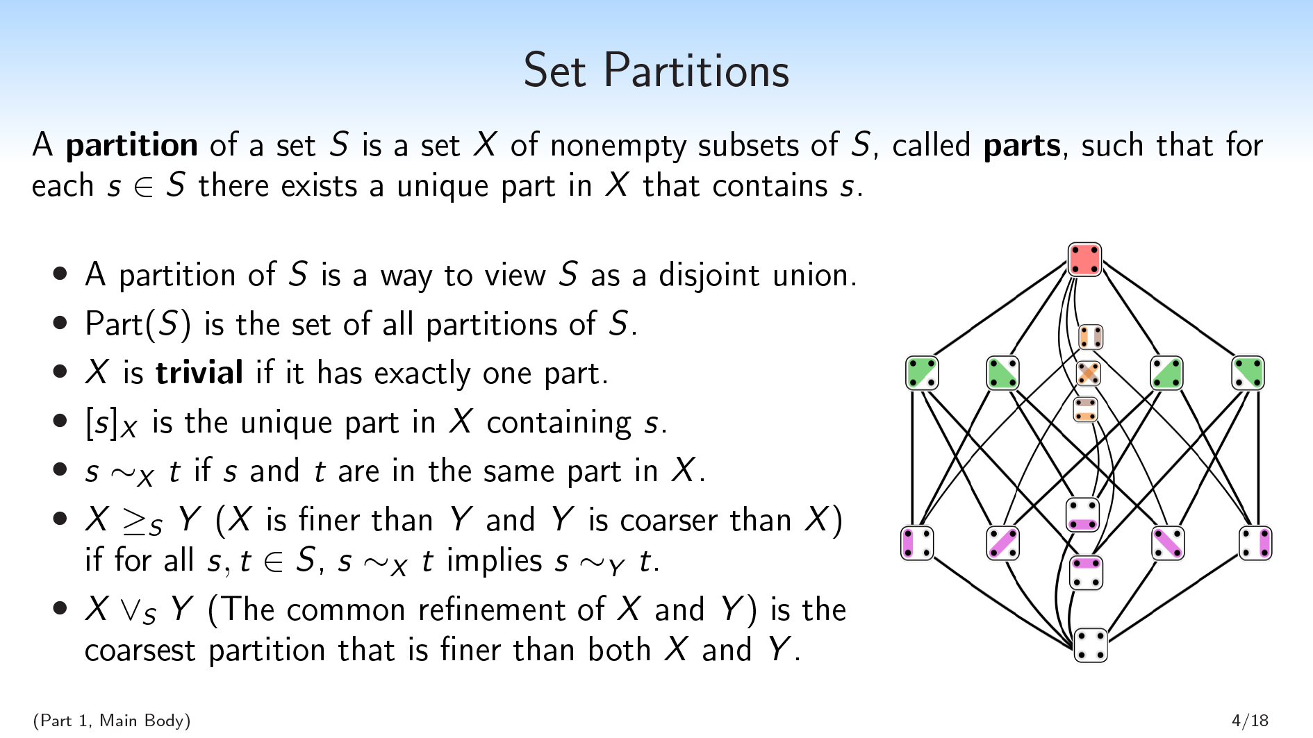
- 一种划分of a set \(S\) is a set \(X\) of non-empty subsets of \(S\), calledparts,,,,such that for each \(s∈S\) there exists a unique part in \(X\) that contains \(s\).
- Basically, a partition of \(S\) is a way to view \(S\) as a disjoint union. We have parts that are disjoint from each other, and they union together to form \(S\).
- 我们将为\(s \)的所有分区编写\(\ mathrm {part}(s)\)。
- We’ll say that a partition \(X\) istrivialif it has exactly one part.
- We’ll use bracket notation, \([s]_{X}\), to denote the unique part in \(X\) containing \(s\). So this is like the equivalence class of a given element.
- 我们将使用符号\(s〜_ {x} t \)说两个元素\(s \)和\(t \)在\(x \)中的同一部分。
您还可以将分区视为集合\(s \)上的变量。以这种方式查看,分区的值\(x \)对应于元素在哪个部分中。
或者,您可以将\(x \)视为一个题您可以询问\(s \)的通用元素。如果我有一个\(s \)的元素,并且它对您隐藏,并且您想问一个问题,则每个可能的问题都对应于根据不同可能的答案分割\(s \)的分区。
We’re also going to use thelattice structureof partitions:
- We’ll say that \(X \geq_S Y\) (\(X\) is finer than \(Y\), and \(Y\) is coarser than \(X\)) if \(X\) makes all of the distinctions that \(Y\) makes (and possibly some more distinctions), i.e., if for all \(s,t \in S\), \(s \sim_X t\) implies \(s \sim_Y t\). You can break your set \(S\) into parts, \(Y\), and then break it into smaller parts, \(X\).
- \(X\vee_S Y\) (the common refinement of \(X\) and \(Y\) ) is the coarsest partition that is finer than both \(X\) and \(Y\) . This is the unique partition that makes all of the distinctions that either \(X\) or \(Y\) makes, and no other distinctions. This is well-defined, which I’m not going to show here.
希望这主要是背景。现在我想展示一些新东西。
(第1部分,主体)···设定因素化
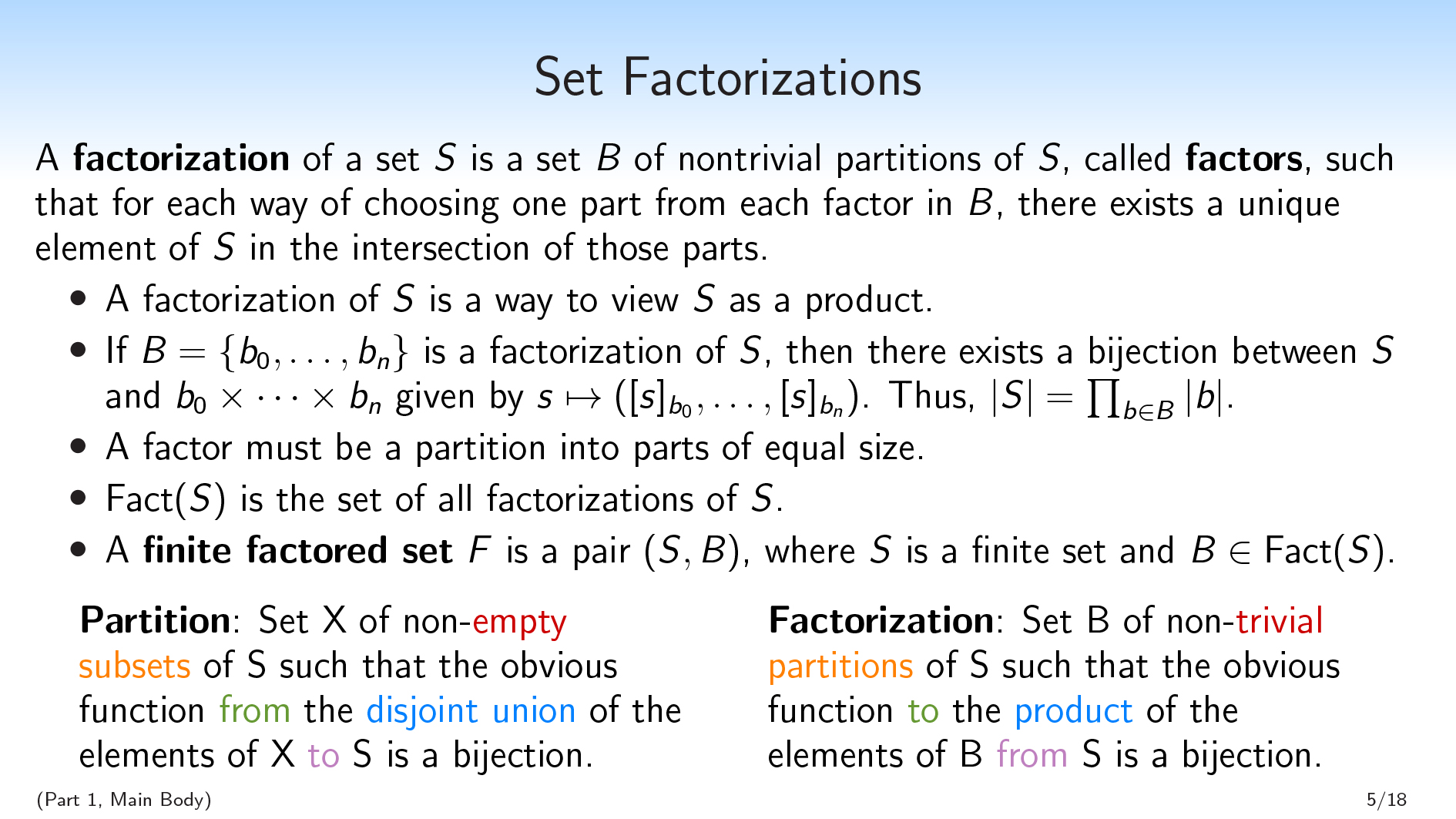 一种分解of a set \(S\) is a set \(B\) of nontrivial partitions of \(S\), called因素,因此,对于从\(b \)中每个因素中选择一个部分的每种方式,在这些部分的相交中存在\(s \)的唯一元素。
因此,这可能有点密集。我对此的简短标语是:“ \(s \)的分解是将\(s \)视为产品的一种方法,就像分区是一种将\(s \)视为一种方式的方式一样脱节联盟。”
If you take one definition away from this first talk, it should be the definition of factorization. I’ll try to explain it from a bunch of different angles to help communicate the concept.
If \(B=\{b_0,\dots,b_{n}\}\) is a factorization of \(S\) , then there exists a bijection between \(S\) and \(b_0\times\dots\times b_{n}\) given by \(s\mapsto([s]_{b_0},\dots,[s]_{b_{n}})\). This bijection comes from sending an element of \(S\) to the tuple consisting only of parts containing that element. And as a consequence of this bijection, \(|S|=\prod_{b\in B} |b|\).
So we’re really viewing \(S\) as a product of these individual factors, with no additional structure.
一种lthough we won’t prove this here, something else you can verify about factorizations is that all of the parts in a factor have to be of the same size.
We’ll write \(\mathrm{Fact}(S)\) for the set of all factorizations of \(S\), and we’ll say that afinite factored set是a pair \((S,B)\), where \(S\) is a finite set and \(B \in \mathrm{Fact}(S)\).
Note that the relationship between \(S\) and \(B\) is somewhat loopy. If I want to define a factored set, there are two strategies I could use. I could first introduce the \(S\), and break it into factors. Alternatively, I could first introduce the \(B\).一种nytime I have a finite collection of finite sets \(B\), I can take their product and thereby produce an \(S\), modulo the degenerate case where some of the sets are empty. So \(S\) can just be the product of a finite collection of arbitrary finite sets.
To my eye, this notion of factorization is extremely natural. It’s basically the multiplicative analog of a set partition. And I really want to push that point, so here’s another attempt to push that point:
| 一种划分是a set \(X\) of非空 子集of \(S\) such that the obvious functionfrom这d是joint unionof \(x \)的元素到\(S\) is a bijection. |
一种分解是一组\(b \)的non-trivial 划分sof \(S\) such that the obvious function到这产品of \(b \)的元素from\(S\) is a bijection. |
我可以从之前对分区定义进行稍微修改的版本,并将一堆单词双重化,并删除设定的分解定义。
希望您现在有点相信这是一个非常自然的概念。
| 安德鲁·克里奇(Andrew Critch):从某种意义上说,斯科特(Scott)将“子集”视为对分区的双重分区,我认为这是有效的。然后,从另一个意义上讲,您将“分解”视为分区双重的。这些都是有效的,但也许值得谈论两种双重性。 斯科特:是的。I think what’s going on there is that there are two ways to view a partition. You can view a partition as “that which is dual to a subset,” and you can also view a partition as something that is built up out of subsets. These two different views do different things when you dualize. Ramana Kumar:I was just going to check: You said you can start with an arbitrary \(B\) and then build the \(S\) from it. It can be literally any set, and then there’s always an \(S\)… 斯科特:如果没有一个是空的,是的,您只能取一组任意元素的集合。您可以采用它们的产品,您可以识别一组元素的每个元素。 Ramana Kumar:一种h. So the \(S\) in that case will just be tuples. 斯科特:那就对了。 Brendan Fong:Scott, given a set, I find it very easy to come up with partitions. But I find it less easy to come up with factorizations. Do you have any tricks for…? 斯科特:为此,我可能应该继续进行示例。 Joseph Hirsh:Can I ask one more thing before you do that? You allow factors to have one element in them? 斯科特:我说“非平凡”,这意味着它没有一个要素。 Joseph Hirsh:“Nontrivial” means “not have one element, and not have no elements”? 斯科特:不,空套有一个分区(没有零件),我将其称为非平地。但是空的东西并不是那么关键。 |
I’m now going to move on to some examples.
(第1部分,示例)···Enumerating Factorizations
Exercise! What are the factorizations of the set \(\{0,1,2,3\}\) ?
Spoiler space:
。
。
。
。
。
。
。
。
。
。
。
。
。
。
 首先,我们将有一种琐碎的分解:
\(\begin{split} \{ \ \ \{ \{0\},\{1\},\{2\},\{3\} \} \ \ \} \end{split} \begin{split} \ \ \ \ \underline{\ 0 \ \ \ 1 \ \ \ 2 \ \ \ 3 \ } \end{split}\)
我们只有一个因素,该因素是离散分区。只要您的集合至少有两个元素,您就可以为任何集合做到这一点。
Recall that in the definition of factorization, we wanted that for each way of choosing one part from each factor, we had a unique element in the intersection of those parts. Since we only have one factor here, satisfying the definition just requires that for each way of choosing one part from the discrete partition, there exists a unique element that is in that part.
然后我们想要一些琐碎的分解。In order to have a factorization, we’re going to need some partitions. And the product of the cardinalities of our partitions are going to have to equal the cardinality of our set \(S\) , which is 4.
表达4作为非平凡产品的唯一方法是将其表示为\(2 \ times 2 \)。因此,我们正在寻找具有2个因素的因素化,每个因素都有2个部分。
我们早些时候注意到,一个因素中的所有零件都必须具有相同的大小。因此,我们正在寻找2个分区,每个分区将我们的4个元素设置分成2组2组。
So if I’m going to have a factorization of \(\{0,1,2,3\}\) that isn’t this trivial one, I’m going to have to pick 2 partitions of my 4-element set that each break the set into 2 parts of size 2. And there are 3 partitions of a 4-element sets that break it up into 2 parts of size 2. For each way of choosing a pair of these 3 partitions, I’m going to get a factorization.
\(\begin{split} \begin{Bmatrix} \ \ \ \{\{0,1\}, \{2,3\}\}, \ \\ \{\{0,2\}, \{1,3\}\} \end{Bmatrix} \end{split} \begin{split} \ \ \ \ \ \ \ \ \ \ \ \ \ \ \ \ \begin{array} { |c|c|c|c| } \hline 0 & 1 \\ \hline 2 & 3 \\ \hline \end{array} \end{split}\)
\(\ begin {split} \ begin {bmatrix} \ \ \ \ \ {\ {\ {0,1 \},\ {2,3 \} \},\ \ \ \ \ \ {\ {\ {0,3 \}1,,,,2\}\} \end{Bmatrix} \end{split} \begin{split} \ \ \ \ \ \ \ \ \ \ \ \ \ \ \ \ \begin{array} { |c|c|c|c| } \hline 0 & 1 \\ \hline 3 & 2 \\ \hline \end{array} \end{split}\)
\(\begin{split} \begin{Bmatrix} \ \ \ \{\{0,2\}, \{1,3\}\}, \ \\ \{\{0,3\}, \{1,2\}\} \end{Bmatrix} \end{split} \begin{split} \ \ \ \ \ \ \ \ \ \ \ \ \ \ \ \ \begin{array} { |c|c|c|c| } \hline 0 & 2 \\ \hline 3 & 1 \\ \hline \end{array} \end{split}\)
So there will be 4 factorizations of a 4-element set.
In general you can ask, “How many factorizations are there of a finite set of size \(n\) ?”. Here’s a little chart showing the answer for \(n \leq 25\):
| \(| s | \) | \(| \ mathrm {fact}(s)| \) |
| 0 | 1 |
| 1 | 1 |
| 2 | 1 |
| 3 | 1 |
| 4 | 4 |
| 5 | 1 |
| 6 | 61 |
| 7 | 1 |
| 8 | 1681年 |
| 9 | 5041 |
| 10 | 15121 |
| 11 | 1 |
| 12 | 13638241 |
| 13 | 1 |
| 14 | 8648641 |
| 15 | 1816214401 |
| 16 | 181880899201 |
| 17 | 1 |
| 18 | 45951781075201 |
| 19 | 1 |
| 20 | 3379365788198401 |
| 21 | 1689515283456001 |
| 22 | 14079294028801 |
| 23 | 1 |
| 24 | 4454857103544668620801 |
| 25 | 538583682060103680001 |
You’ll notice that if \(n\) is prime, there will be a single factorization, which hopefully makes sense. This is the factorization that only has one factor.
在我看来,一个非常令人惊讶的事实是,这个序列没有出现OEIS,,,,which is this database that combinatorialists use to check whether or not their sequence has been studied before, and to see connections to other sequences.
对我来说,这感觉就像Bell numbers。钟数计算了有多少个大小\(n \)的分区。OEI的序列编号为110,超过300,000;而且,即使我对其进行调整并删除了堕落的案例,依此类推,这个序列根本不会出现。
我对这个事实感到非常困惑。对我来说,因素化似乎是一个非常自然的概念,在我看来,它似乎以前从未真正被研究过。
这是我简短的组合演讲的终结。
| Ramana Kumar:If you’re willing to do it, I’d appreciate just stepping through one of the examples of the factorizations and the definition, because this is pretty new to me. 斯科特:是的。Let’s go through the first nontrivial factorization of \(\{0,1,2,3\}\): \(\begin{split} \begin{Bmatrix} \ \ \ \{\{0,1\}, \{2,3\}\}, \ \\ \{\{0,2\}, \{1,3\}\} \end{Bmatrix} \end{split} \begin{split} \ \ \ \ \ \ \ \ \ \ \ \ \ \ \ \ \begin{array} { |c|c|c|c| } \hline 0 & 1 \\ \hline 2 & 3 \\ \hline \end{array} \end{split}\) In the definition, I said a factorization should be a set of partitions such that for each way of choosing one part from each of the partitions, there will be a unique element in the intersection of those parts. 在这里,我有一个分区,将小数字与大数字分开:\(\ {\ {0,1 \},\ {2,3 \} \} \)。而且我还有一个分区,将偶数数字与奇数数分开:\(\ {\ {0,2 \},\ {1,3 \} \} \)。 一种nd the point is that for each way of choosing either “small” or “large” and also choosing “even” or “odd”, there will be a unique element of \(S\) that is the conjunction of these two choices. In the other two nontrivial factorizations, I replace either “small and large” or “even and odd” with an “inner and outer” distinction. David Spivak:对于分区和许多事情,如果我知道集合\(a \)的分区和集合\(b \)的分区,那么我知道\(a+b \)的一些分区(不相关联合会)或者我知道\(a \ times b \)的一些分区。您知道有什么事实以进行因素化吗? 斯科特:是的。If I have two factored sets, I can get a factored set over their product, which sort of disjoint-unions the two collections of factors. For the additive thing, you’re not going to get anything like that because prime sets don’t have any nontrivial factorizations. |
好的。我想我将继续进行主谈话。
(第2部分,标题幻灯片)···这Main Talk (It’s About Time)
((Part 2, Motivation) · · ·这Pearlian Paradigm
 我们不能不谈论时间谈论时间珍珠因果推断。我想开始说我认为珍珠型很棒。这给我买了一些crackpot点,但我要说的是自爱因斯坦以来时间的理解,这是最好的事情。
我不会在这里介绍珍珠范式的所有细节。我的演讲在技术上不会取决于它;这是为了动力。
Given a collection of variables and a joint probability distribution over those variables, Pearl can infer causal/temporal relationships between the variables. (In this talk I’m going to use “causal” and “temporal” interchangeably, though there may be more interesting things to say here philosophically.)
Pearl can infer temporal data from statistical data, which is going against the adage that “correlation does not imply causation.” It’s like Pearl is taking the combinatorial structure of your correlation and using that to infer causation, which I think is just really great.
| Ramana Kumar:I may be wrong, but I think this is false. Or I think that that’s not all Pearl needs—just the joint distribution over the variables. Doesn’t he also make use of intervention distributions? 斯科特:In the theory that is described in chapter two of the book因果关系,他并没有真正使用其他东西。珍珠在其他地方建立了这个更大的理论。但是,您具有很强的能力,也许假设简单性或其他任何东西(但没有假设您可以访问额外的信息),可以收集变量和对这些变量的联合分布,并从相关性中推断出因果关系。 安德鲁·克里奇(Andrew Critch):Ramana, it depends a lot on the structure of the underlying causal graph. For some causal graphs, you can actually recover them uniquely with no interventions. And only assumptions with zero-measure exceptions are needed, which is really strong. Ramana Kumar:Right, but then the information you’re using is the graph. 安德鲁·克里奇(Andrew Critch):No, you’re not. Just the joint distribution. Ramana Kumar:哦好的。抱歉,继续。 安德鲁·克里奇(Andrew Critch):这re exist causal graphs with the property that if nature is generated by that graph and you don’t know it, and then you look at the joint distribution, you will infer with probability 1 that nature was generated by that graph, without having done any interventions. Ramana Kumar:Got it. That makes sense. Thanks. 斯科特:凉爽的。 |
不过,我要(一点)反对这一点。我要声称那个珍珠是kind of cheating when making this inference. The thing I want to point out is that in the sentence “Given a collection of variables and a joint probability distribution over those variables, Pearl can infer causal/temporal relationships between the variables.”, the words “Given a collection of variables” are actually hiding a lot of the work.
重点通常放在联合probability distribution, but Pearl is not inferring temporal data from statistical data alone. He is inferring temporal data from statistical data和分解数据:如何将世界分解为这些变量。
我声称这个问题也与未能充分处理抽象和确定论的情况纠缠在一起。要指出这一点,可以做类似说的事情:
“Well, what if I take the variables that I’m given in a Pearlian problem and I just forget that structure? I can just take the product of all of these variables that I’m given, and consider the space of all partitions on that product of variables that I’m given; and each one of those partitions will be its own variable. And then I can try to do Pearlian causal inference on this big set of all the variables that I get by forgetting the structure of variables that were given to me.”
问题在于,当您这样做时,您会有很多彼此确定的功能,并且实际上无法使用Pearlian Paradigm推断出东西。
So in my view, this cheating is very entangled with the fact that Pearl’s paradigm isn’t great for handling abstraction and determinism.
((Part 2, Table of Contents) · · ·We Can Do Better
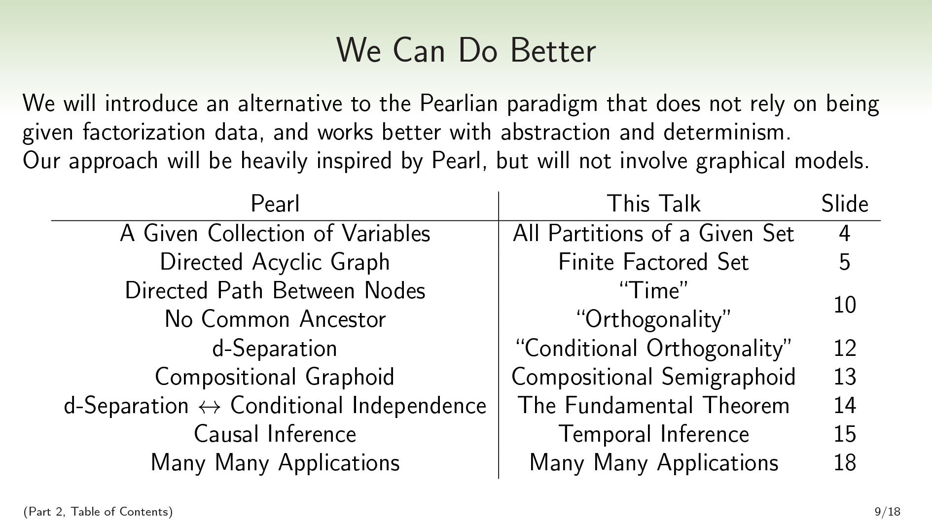 在这次演讲中,我们将要做的主要工作是我们将介绍不依赖分解数据的珍珠的替代方案,因此在抽象和确定性方面更好地效果。
Where Pearl was given a collection of variables, we are going to just consider all partitions of a given set. Where Pearl infers a directed acyclic graph, we’re going to infer a finite factored set.
In the Pearlian world, we can look at the graph and read off properties of time and orthogonality/independence. A directed path between nodes corresponds to one node being before the other, and two nodes are independent if they have no common ancestor. Similarly, in our world, we will be able to read time and orthogonality off of a finite factored set.
((Orthogonality and independence are pretty similar. I’ll use the word “orthogonality” when I’m talking about a combinatorial notion, and I’ll use “independence” when I’m talking about a probabilistic notion.)
In the Pearlian world,d- 您可以从图表中读取的分离,对应于可以放在图表上的所有概率分布中的条件独立性。我们将拥有一个基本的定理,它基本上是同一件事:条件正交性对应于我们可以将其放在各种概率分布中的条件独立性。
In the Pearlian world,d- 分离将满足组成图型公理。在我们的世界中,我们将满足构图半径公理。我声称您首先不应该想要的第五章图形公理。
珍珠做因果推断。我们将讨论如何使用这种新范式进行时间推理,并推断出珍珠方法无法做到的一些非常基本的时间事实。(请注意,珍珠有时也可以推断出时间关系we不能 - 但仅从我们的角度来看,珍珠正在做出其他分解假设。)
一种nd then we’ll talk about a bunch of applications.
| Pearl | 这个谈话 |
| 一种Given Collection of Variables | 给定集的所有分区 |
| 定向无环图 | 有限的委托集 |
| Directed Path Between Nodes | “Time” |
| 没有共同的祖先 | “Orthogonality” |
| d-Separation | “有条件的正交性” |
| Compositional Graphoid | Compositional Semigraphoid |
| d- 分离↔有条件独立性 | 基本定理 |
| Causal Inference | Temporal Inference |
| Many Many Applications | Many Many Applications |
Excluding the motivation, table of contents, and example sections, this table also serves as an outline of the two talks. We’ve already talked about set partitions and finite factored sets, so now we’re going to talk about time and orthogonality.
((Part 2, Main Body) · · ·Time and Orthogonality
 I think that if you capture one definition from this second part of the talk, it should be this one. Given a finite factored set as context, we’re going to define the history of a partition.
令\(f =(s,b)\)为有限的分组集。并让\(x,y \ in \ mathrm {part}(s)\)为\(s \)的分区。
这history\(x \)的书面\(h^f(x)\)是最小的因素\(h \ subseteq b \),因此,如果\(s,t \ in s \),则(s \ sim_b t \)对于所有\(b \ in H \),然后\(s \ sim_x t \)。
那么,\(x \)的历史是最小的因素\(h \) - 因此,是\(b \)的最小子集 - 如果我采用\(s \)的元素,并且向您隐藏它,您想知道它在\(x \)中的哪一部分,这足以告诉您\(H \)中的每个因素中的哪一部分。
So the history \(H\) is a set of factors of \(S\) , and knowing the values of all the factors in \(H\) is sufficient to know the value of \(X\) , or to know which part in \(X\) a given element is going to be in. I’ll give an example soon that will maybe make this a little more clear.
然后我们要定义timefrom history. We’ll say that \(X\) isweakly before\(y \),书面\(x \ leq^f y \),如果\(h^f(x)\ subseteq h^f(y)\)。我们会说\(x \)是strictly before\(Y\), written \(X<^F Y\), if \(h^F(X)\subset h^F(Y)\).
一个类比可以绘制的是,这些历史就像时空中一个点的过去光锥一样。当一个点在另一个点之前,那么早期点的向后光锥将成为后面点的向后光锥的子集。这有助于说明为什么“以前”就像子集的关系。
We’re also going to define orthogonality from history. We’ll say that two partitions \(X\) and \(Y\) areorthogonal,书面\(x \ perp^fy \),如果他们的历史是不相交的:\(h^f(x)\ cap h^f(y)= \ {\ {\} \)。
Now I’m going to go through an example.
((Part 2, Examples) · · ·Game of Life
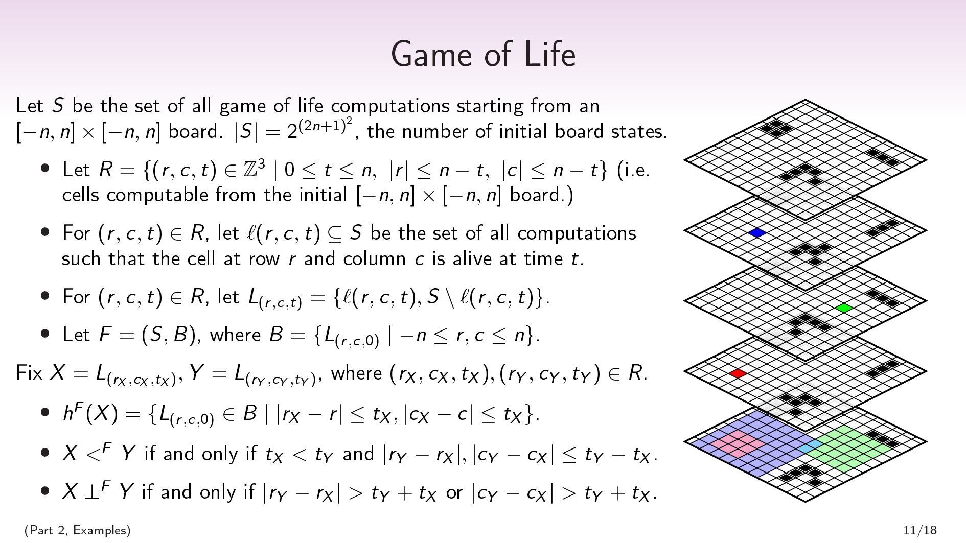 Let \(S\) be the set of all Game of Life computations starting from an \([-n,n]\times[-n,n]\) board.
LET \(r = \ {(r,c,t)\ in \ mathbb {z}^3 \ mid0 \ leq t \ leq t \ leq n,\ \ \ \ \)n-t \} \)(即,可以从初始\([ - n,n] \ times [-n,n] \)板上计算的单元格。对于\((r,c,t)\ in r \),让\(\ ell(r,c,t)\ subseteq s \)是所有计算的集合,使得row \(r \)的单元格(r \)和列\(c \)在时间\(t \)中还活着。
((Minor footnote: I’ve done some small tricks here in order to deal with the fact that the Game of Life is normally played on an infinite board. We want to deal with the finite case, and we don’t want to worry about boundary conditions, so we’re only going to look at the cells that are uniquely determined by the initial board. This means that the board will shrink over time, but this won’t matter for our example.)
\(s \)是生命计算的所有游戏集合,但是由于生命游戏是确定性的,因此所有计算的集合都与所有初始条件的集合中均属于Berijective对应关系。\(| s | = 2^{(2n+1)^{2}} \),初始板的数量。
This also gives us a nice factorization on the set of all Game of Life computations. For each cell, there’s a partition that separates out the Game of Life computations in which that cell is alive at time 0 from the ones where it’s dead at time 0. Our factorization, then, will be a set of \((2n+1)^{2}\) binary factors, one for each question of “Was this cell alive or dead at time 0?”.
形式上:for \(((r,c,t)\ in r \),让\(l _ {(r,c,t)} = \ {\ ell(r,c,t),s \ setMinus \ ell(r,c,t)\} \)。令\(f =(s,b)\),其中\(b = \ {l _ {(r,c,0)} \ mid -n \ leq r,c \ leq n \} \)。
我们可以谈论的所有生命计算游戏中还将有其他分区。例如,您可以拿一个单元格和一个时间\(t \)说:“这个单元格在时间\(t \)?at time \(t\) from the computations where it’s dead at time \(t\).
这是一个例子:
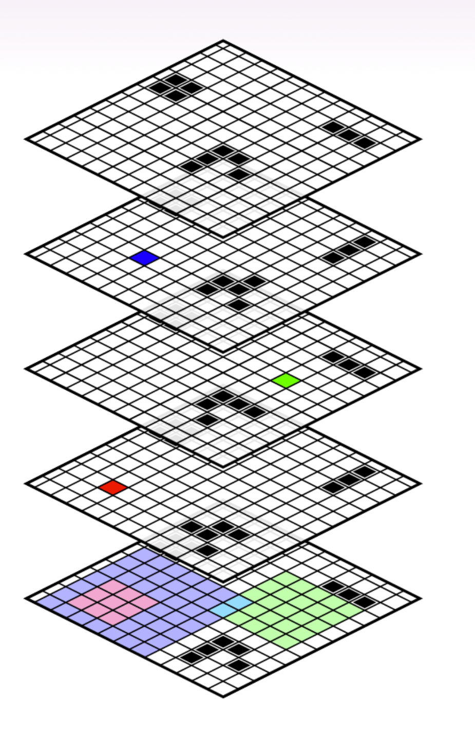
最低网格显示了初始董事会状态的一部分。
上板上的蓝色,绿色和红色正方形是(时间)对。每个广场都对应于所有生命计算游戏集的分区:“该单元格是在给定时间\(t \)的生存还是死亡?”
这history of that partition is going to be all the cells in the initial board that go into computing whether the cell is alive or dead at time \(t\) . It’s everything involved in figuring out that cell’s state. E.g., knowing the state of the nine light-red cells in the initial board always tells you the state of the red cell in the second board.
在此示例中,与红细胞状态相对应的分区严格是在与蓝细胞相对应的分区之前。红细胞是活着还是死了的问题是在蓝细胞是活着还是死的问题之前。
Meanwhile, the question of whether the red cell is alive or dead is going to beorthogonal到这题of whether the green cell is alive or dead.
一种nd the question of whether the blue cell is alive or dead isnot与绿细胞是活着还是死亡的问题是正交的,因为它们在青色细胞上相交。
概括点,fix \(x = l _ {(r_x,c_x,t_x)},y = l _ {(r_y,c_y,t_y)} \),其中\(r_x,c_x,t_x),(r_y,c_y,c_y,c_y,c_y,c_y,t_y)\ in r \)。然后:
- \(h^{F}(X)=\{L_{(r,c,0)}\in B\mid |r_X-r|\leq t_X,|c_X-c|\leq t_X\}\).
- \(X \ ᐸ^{F} \ Y\) if and only if \(t_X \ ᐸ \ t_Y\) and \(|r_Y-r_X|,|c_Y-c_X|\leq t_Y-t_X\).
- \(x \ perp^f y \)if and&hork if \(| r_y-r_x |> t_y+t_x \)或\(| c_y-c_x |> t_y+t_x \)。
我们还可以看到蓝色和绿色细胞看起来艾尔most正交。如果我们在其历史的交集中根据两个青色细胞的值进行条件,则然后蓝色和绿色分区变为正交。这就是我们接下来要讨论的内容。
| David Spivak:一种priori, that would be a gigantic computation—to be able to tell me that you understand the factorization structure of that Game of Life. So what intuition are you using to be able to make that claim, that it has the kind of factorization structure you’re implying there? 斯科特:So, I’ve defined the factorization structure. David Spivak:您已经给了我们一定的分解。因此,您对您有很好的直觉history,,,,I guess. Maybe that’s what I’m asking about. 斯科特:是的。因此,如果我不给您分解,那么您可以在这里进行的这种令人讨厌的因素化。然后,对于历史记录,我正在使用的直觉是:“为了计算这个值,我需要知道什么?” 我实际上经历了,我在生活游戏中做了一些小工具,以确保我就在这里,在某些情况下,每个单元都可以影响所讨论的细胞。但是,是的,我从中工作的直觉主要是关于计算中的信息。这是“我可以构建一个情况,如果我知道这个事实,我就能计算出该价值是什么?如果我不能,那么它可能需要两个不同的值。” David Spivak:好的。我认为从定义中得出这种直觉是我缺少的,但是我不知道我们是否有时间经历。 斯科特:Yeah, I think I’m not going to here. |
((Part 2, Main Body) · · ·Conditional Orthogonality
 因此,只是为了设定您的期望:每次我向某人解释珍珠因果的推论时,他们都会说d-separation is the thing they can’t remember.d- 分离是一个比“节点之间的定向路径”和“没有任何共同祖先的节点”的概念要复杂得多。同样,有条件的正交性将比我们的范式中的时间和正交性复杂得多。尽管我确实认为有条件的正交性具有比d-separation.
We’ll begin with the definition of conditional history. We again have a fixed finite set as our context. Let \(F=(S,B)\) be a finite factored set, let \(X,Y,Z\in\text{Part}(S)\), and let \(E\subseteq S\).
\(x \)给定\(e \)的条件历史,书面\(h^f(x | e)\)是满足以下两个条件的最小因子\(h \ subseteq b \)的最小因素集:
- 对于所有\(s,t \ in e \),如果\(s \ sim_ {b} t \)对于所有\(b \ in H \),则\(s \ sim_x t \)。
- 对于所有\(s,t \ in e \)和\(r \ in s \),如果\(r \ sim__ {b_0} s \)for all \(b_0 \ in H \)和\(r \ sim_{b_1} t \)for ash as ash \(b_1 \ in B \ setminus h \),然后\(r \ in e \)。
第一个条件是很像的条件had in our definition of history, except we’re going to make the assumption that we’re in \(E\). So the first condition is: if all you know about an object is that it’s in \(E\), and you want to know which part it’s in within \(X\), it suffices for me to tell you which part it’s in within each factor in the history \(H\).
我们的第二个条件实际上并不是要提及\(x \)。这将是\(e \)和\(h \)之间的关系。它说,如果您想弄清楚(s \)的元素是否在\(e \)中,则足以并行化并提出两个问题:
- “If I only look at the values of the factors in \(H\), is ‘this point is in \(E\)’ compatible with that information?”
- “If I only look at the values of the factors in \(B\setminus H\) , is ‘this point is in \(E\)’ compatible with that information?”
If both of these questions return “yes”, then the point has to be in \(E\).
我不会就为什么需要成为定义的一部分的直觉。我要说的是,如果没有第二种条件,有条件的历史甚至都不会得到很好的定义,因为在交集下不会关闭它。因此,我将无法在子集排序中采用最小的因素。
与其通过解释其背后的直觉来证明这一定义是合理的,我将通过使用并吸引其后果来证明它是合理的。
We’re going to use conditional history to defineconditional orthogonality,,,,just like we used history to define orthogonality. We say that \(X\) and \(Y\) are给出正交\(e \ subseteq s \),书面\(x \ perp^{f} y \ mid e \),如果\(x \)给定\(e \)的历史与\的历史不相交(y(y)\)给定\(e \):\(h^f(x | e)\ cap h^f(y | e)= \ {\} \)。
We say \(X\) and \(Y\) are给出正交\(z \ in \ text {part}(s)\),书面\(x \ perp^{f} y \ mid z \),如果\(x \ perp^{f} y mid z \)全\(z \ in z \)。因此,考虑到分区的每种单独的方式,该分区可能是该分区中的每个单个部分,就意味着成为正交的是正交的。
我已经使用了一段时间了,对我来说感觉很自然,但是我没有很好的方法来推动这种情况的自然性。因此,我再次想吸引后果。
((Part 2, Main Body) · · ·组成半径公理
 有条件的正交满足组成半径公理,,,,which means finite factored sets are pretty well-behaved.
令\(f =(s,b)\)为有限的委托集,让\(x,y,z,w \ in \ text {part}(s)\)为\(s \)的分区。然后:
- If \(X \perp^{F} Y \mid Z\), then \(Y \perp^{F} X \mid Z\). (symmetry)
- 如果\ \(x \ perp^{f}(y \ vee_s w)\ mid z \),则\(x \ perp^{f} y \ mid z \)和\(x \ perp^{f} w \ \ perp^{f}中部Z \)。((decomposition)
- If \(X \perp^{F} (Y\vee_S W) \mid Z\), then \(X \perp^{F} Y \mid (Z\vee_S W)\). (weak union)
- if \(x \ perp^{f} y \ mid z \)和\(x \ perp^{f} w \ mid(z \ vee_s y)\),然后\(x \ perp^{f}(y\ vee_s w)\中Z \)。((contraction)
- if \(x \ perp^{f} y \ mid z \)和if \(x \ perp^{f} w \ mid z \),然后\(x \ perp^{f}(y \ vee_s w)\中Z \)。((作品)
这first four properties here make up the semigraphoid axioms, slightly modified because I’m working with partitions rather than sets of variables, so union is replaced with common refinement. There’s another graphoid axiom which we’re not going to satisfy; but I argue that we don’t want to satisfy it, because it doesn’t play well with determinism.
这里的第五个属性(构图)也许是最直觉的属性之一,因为它并不完全受到概率独立性的满足。
Decomposition and composition act like converses of each other. Together, conditioning on \(Z\) throughout, they say that \(X\) is orthogonal to both \(Y\) and \(W\) if and only if \(X\) is orthogonal to the common refinement of \(Y\) and \(W\).
((Part 2, Main Body) · · ·基本定理
 除了表现良好之外,我还想证明有条件的正交性非常强大。我想做的方式是通过显示条件正交性与有限分布的所有概率分布中的条件独立性完全相对应。因此,很像d- 在珍珠图中分离,有条件的正交性可以视为概率独立性的组合版本。
一种probability distribution on a finite factored set\(F=(S,B)\) is a probability distribution \(P\) on \(S\) that can be thought of as coming from a bunch of independent probability distributions on each of the factors in \(B\). So \(P(s)=\prod_{b\in B}P([s]_b)\) for all \(s\in S\).
这有效地意味着您的概率分布因素与设定因素相同:任何给定元素的概率是每个因素内部每个零件的概率的乘积。
这fundamental theorem of finite factored sets说:让\(f =(s,b)\)为有限的委托集,让\(x,y,z \ in \ text {part}(s)\)为\(s \)的分区。然后,\(x \ perp^{f} y \ mid z \),并且仅在\(f \)上所有概率分布\(p \),以及all \(x \ in x \),\(y(y)\ in y \)和\(z \ in z \),我们有\(p(x \ cap z)\ cdot p(y \ cap z)= p(x \ cap y \ cap z)\ cdot p(z)\)。即,如果在所有概率分布中满足\(z \)给定的\(z \),则与\(y \)之间是正交的。在所有概率分布中。
This theorem, for me, was a little nontrivial to prove. I had to go through defining certain polynomials associated with the subsets, and then dealing with unique factorization in the space of these polynomials; I think the proof was eight pages or something.
这fundamental theorem allows us to infer orthogonality data from probabilistic data. If I have some empirical distribution, or I have some Bayesian distribution, I can use that to infer some orthogonality data. (We could also imagine orthogonality data coming from other sources.) And then we can use this orthogonality data to get temporal data.
So next, we’re going to talk about how to get temporal data from orthogonality data.
((Part 2, Main Body) · · ·Temporal Inference
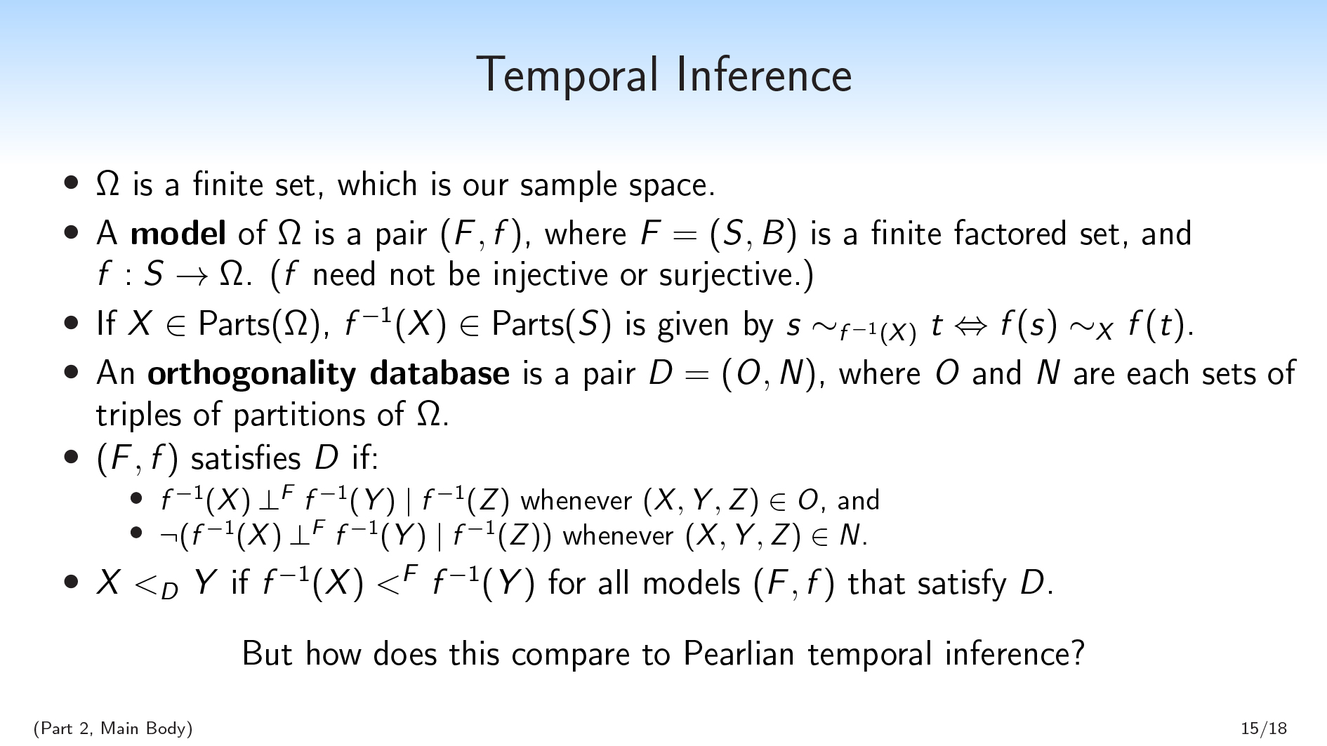 我们将从有限集\(\ omega \)开始,这是我们的样本空间。
您可能会认为我们会尝试做的一件天真的事情是推断\(\ omega \)的分解。我们不会这样做,因为那将太过限制。我们要允许\(\ omega \)向我们隐藏一些信息,以便有一些潜在的结构等。
这re may be some situations that are distinct without being distinct in \(\Omega\). So instead, we’re going to infer a factored set model of \(\Omega\): some other set \(S\), and a factorization of \(S\), and a function from \(S\) to \(\Omega\).
一种model of \(\Omega\) is a pair \((F, f)\), where \(F=(S,B)\) is a finite factored set and \(f:S\rightarrow \Omega\). ( \(f\) need not be injective or surjective.)
然后,如果我有一个\(\ omega \)的分区,则可以在\(f \)上向后发送此分区,并获得\(s \)的唯一分区。如果\(x \ in \ text {parts}(\ omega)\),则\(f^{ - 1}(x)(x)\ in \ text {parts}(s)\)由\(s \ sim_{f^{ - 1}(x)} t \ leftrightArrow f(s)\ sim_x f(t)\)。
那么,我们要做的就是采取有关\(\ omega \)的一堆正交性事实,我们将尝试找到一个捕获正交性事实的模型。
我们将给出一个orthogonality database在\(\ omega \)上,这是一对(d =(o,n)\),其中\(o \)(对于“正交”)和\(n \)(对于“非正交”)是\(\ omega \)的分区的每组\((x,y,z)\)。我们将这些视为关于正交性的规则。
对于模型\((f,f)\)满足数据库\(d \)的含义是:
- \(f^{ - 1}(x)\ perp^{f} f^{ - 1}(y)\ mid f^{ - 1}(z)\)e时在o \)和
- \(\) \(\lnot (f^{-1}(X) \perp^{F} f^{-1}(Y) \mid f^{-1}(Z))\) whenever \((X,Y,Z)\in N\).
So we have these orthogonality rules we want to satisfy, and we want to consider the space of all models that are consistent with these rules. And even though there will always be infinitely many models that are consistent with my database, if at least one is—you can always just add more information that you then delete with \(f\)—we would like to be able to sometimes infer that for all models that satisfy our database, \(f^{-1}(X)\) is before \(f^{-1}(Y)\).
一种nd this is what we’re going to mean by inferring time. If all of our models \((F,f)\) that are consistent with the database \(D\) satisfy some claim about time \(f^{-1}(X) \ ᐸ^F \ f^{-1}(Y)\), we’ll say that \(X \ ᐸ_D \ Y\).
((Part 2, Examples) · · ·Two Binary Variables (Pearl)
 So we’ve set up this nice combinatorial notion of temporal inference. The obvious next questions are:
- Can we actually infer interesting facts using this method, or is it vacuous?
- 一种nd: How does this framework compare to Pearlian temporal inference?
珍珠时刻的推论确实非常强大。给定足够的数据,它可以在各种情况下推断时间序列。相比之下,有限的体内设置方法有多强大?
To address that question, we’ll go to an example. Let \(X\) and \(Y\) be two binary variables. Pearl asks: “Are \(X\) and \(Y\) independent?” If yes, then there’s no path between the two. If no, then there may be a path from \(X\) to \(Y\), or from \(Y\) to \(X\), or from a third variable to both \(X\) and \(Y\).
无论哪种情况,我们都不会推断任何时间关系。
对我来说,感觉就像这是“相关性不暗示因果关系”的地方。珍珠确实需要更多的变量,以便能够从更丰富的组合结构中推断出时间关系。
However, I claim that this Pearlian ontology in which you’re handed this collection of variables has blinded us to the obvious next question, which is: is \(X\) independent of \(X \ \mathrm{XOR} \ Y\)?
In the Pearlian world, \(X\) and \(Y\) were our variables, and \(X \ \mathrm{XOR} \ Y\) is just some random operation on those variables. In our world, \(X \ \mathrm{XOR} \ Y\) instead is a variable on the same footing as \(X\) and \(Y\). The first thing I do with my variables \(X\) and \(Y\) is that I take the product \(X \times Y\) and then I forget the labels \(X\) and \(Y\).
So there’s this question, “Is \(X\) independent of \(X \ \mathrm{XOR} \ Y\)?”. And if \(X\)是独立于\ \(x \ \ mathrm {xor} \ y \),实际上我们将能够得出结论,\(x \)是before\(Y\)!
So not only is the finite factored set paradigm non-vacuous, and not only is it going to be able to keep up with Pearl and infer things Pearl can’t, but it’s going to be able to infer a temporal relationship from only two variables.
So let’s go through the proof of that.
((Part 2, Examples) · · ·两个二进制变量(分组集)
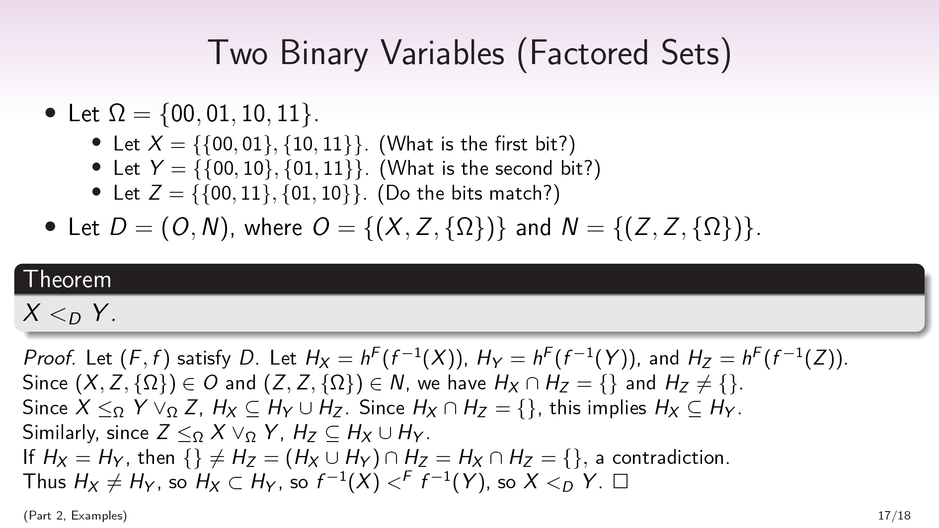
Let \(\Omega=\{00,01,10,11\}\), and let \(X\), \(Y\), and \(Z\) be the partitions (/questions):
- \(x = \ {\ {00,01 \},\ {10,11 \} \} \)。(第一个是什么?)
- \(Y=\{\{00,10\}, \{01,11\}\}\). (What is the second bit?)
- \(Z=\{\{00,11\}, \{01,10\}\}\). (Do the bits match?)
令\(d =(o,n)\),其中\(o = \ {(x,z,z,\ {\ omega \})\} \)和\(n = \ {(z,z,z,z,\ {\ omega \})\} \)。如果我们从概率分布中获得了这个正交性数据库,那么我们将拥有超过两个规则,因为我们会观察到更多的正交性和非正交性。但是,时间推断对于添加更多规则是单调的,因此我们可以处理证明所需的最小规则。
第一个规则说\(x \)与\(z \)正交。第二个规则说\(z \)不是本身正交的,这基本上只是说\(z \)是非确定性的。可以说,\(z \)中的两个部分都是在函数\(f \)下支持的。\(\ {\ omega \} \)表示我们没有任何条件。
From this, we’ll be able to prove that \(X \ ᐸ_D \ Y\).
证明。First, we’ll show that that \(X\) is weakly before \(Y\). Let \((F,f)\) satisfy \(D\). Let \(H_X\) be shorthand for \(h^F(f^{-1}(X))\), and likewise let \(H_Y=h^F(f^{-1}(Y))\) and \(H_Z=h^F(f^{-1}(Z))\).
由于\((x,z,\ {\ omega \})\ in o \),因此我们有那个\(h_x \ cap h_z = \ {\ {\} \);并且由于\((z,z,\ {\ omega \})\在n \),所以我们有那个\(h_z \ neq \ {\} \)。
Since \(X\leq_{\Omega} Y\vee_{\Omega} Z\)—that is, since \(X\) can be computed from \(Y\) together with \(Z\)—\(H_X\subseteq H_Y\cup H_Z\). (Because a partition’s history is the smallest set of factors needed to compute that partition.)
一种nd since \(H_X\cap H_Z=\{\}\), this implies \(H_X\subseteq H_Y\), so \(X\) is weakly before \(Y\).
为了显示严格的不平等,我们将假设出于矛盾的目的,即(h_x \)= \(h_y \)。
请注意,可以与\(y \)一起从\(x \)一起计算\(z \) - 也就是说,\(z \ leq _ {\ omega} x \ vee _ {\ omega} y \) - 因此(h_z \ subseteq H_x \ cup h_y \)(即\(H_z \ subseteq H_x \))。\(h_z =(H_x \ Cup H_Y)\ CAP H_z = H_X \ CAP H_z \)。但是由于\(h_z \)也与\(h_x \)不相交,因此这意味着\(h_z = \ {\} \),矛盾。
Thus \(H_X\neq H_Y\), so \(H_X \subset H_Y\), so \(f^{-1}(X) \ ᐸ^F \ f^{-1}(Y)\), so \(X \ ᐸ_D \ Y\). □
When I’m doing temporal inference using finite factored sets, I largely have proofs that look like this. We collect some facts about emptiness or non-emptiness of various Boolean combinations of histories of variables, and we use these to conclude more facts about histories of variables being subsets of each other.
I have a more complicated example that uses conditional orthogonality, not just orthogonality; I’m not going to go over it here.
我想在这里提出的一个有趣的观点是,我们正在做时间推断 - 我们正在推断\(x \)在\(y \)之前 - 但我声称我们也在做概念上的推断。
Imagine that I had a bit, and it’s either a 0 or a 1, and it’s either blue or green. And these two facts are primitive and independently generated. And I also have this other concept that’s like, “Is it grue or bleen?”, which is the \(\mathrm{XOR}\) of blue/green and 0/1.
从某种意义上说,我们要推断\(x \)在\(y \)之前,在这种情况下,我们可以推断出蓝度在gruense之前。这指出了一个事实,即蓝色更为原始,而Grueness是一种派生的属性。
在我们的证明中,可以将这些原始属性视为\(x \)和\(z \),而\(y \)是我们从中获得的派生属性。因此,我们不仅在推断时间;我们正在推断出关于什么是自然概念的事实。而且我认为,这个本体论可以为“您无法真正区分蓝色和Grue”的说法做一些希望,而Pearl可以对“相关性并不意味着因果关系”做些什么。
((Part 2, Main Body) · · ·申请 /未来工作 /猜测
 我对有限分组集的未来工作属于三个粗略的类别:推理(涉及更多计算问题),无穷大(更多数学)和嵌入式代理(更多哲学)。
Research topics related to inference:
- Decidability of Temporal Inference
- 有效的时间推断
- Conceptual Inference
- Temporal Inference from Raw Data and Fewer Ontological Assumptions
- 与确定关系的时间推断
- 没有正交的时间
- Conditioned Factored Sets
这re are a lot of research directions suggested by questions like “How do we do efficient inference in this paradigm?”. Some of the questions here come from the fact that we’re making fewer assumptions than Pearl, and are in some sense more coming from the raw data.
然后,我有有关将各项集合扩展到无限情况的应用程序:
- Extending Definitions to the Infinite Case
- 有限维的基本定理集合
- 连续的时间
- New Lens on Physics
我在这次演讲中介绍的所有内容都是在有限的假设下。在某些情况下,这不是必需的,但是在很多情况下,我并没有引起人们的注意。
我怀疑可以将基本定理扩展到有限维的分组集(即,\(| b | \)是有限的,但不能将其扩展到任意维定的方面集合。
一种nd then, what I’m really excited about is applications to embedded agency:
- 嵌入式观测
- Counterfactability
- Cartesian FramesSuccessor
- UnravelingCausal Loops
- Conditional Time
- Logical Causality from Logical Induction
- Orthogonality as Simplifying Assumptions for Decisions
- 有条件的正交性作为抽象desideratum
I focused on the temporal inference aspect of finite factored sets in this talk, because it’s concrete and tangible to be able to say, “Ah, we can do Pearlian temporal inference, only we can sometimes infer more structure and we rely on fewer assumptions.”
但是,实际上,我很兴奋的许多应用程序都涉及将有规定的集合用于模型情况,而不是从数据中推断出偏向的集合。
在我们当前使用具有代表信息流或因果关系的有向边缘的图形对情况进行建模的任何地方,我们都可以使用方面的集合来建模情况。这可能会使我们的模型可以通过抽象更出色。
I want to build up the factored set ontology as an alternative to graphs when modeling agents interacting with things, or when modeling information flow. And I’m really excited about that direction.
Did you like this post?You may enjoy our otheryabo app posts, including: